Kaggle's Mercedes Problem: Greedy Selection & Boosting
After our arguably unsuccessful attempt at leveraging PCA to reduce dimensionality, we present throughout this post another approach to the Kaggle’s Mercedes problem that consists in using a forward stepwise feature selection method to reduce the number of features.
We found that with only 4 basic1 features, we can achieve the score of 0.55031 on Kaggle’s LB (and with only 5 features, we obtained 0.55123). That is quite surprising, especially given that, after a one-hot encoding of the categorical variables, there are over 550 features.
Note that we rely on XGBoost for the GBM training, in concert with our own simplistic implementation of a grid search. Due to severe limitations in computational resources, the grid only spans very narrow ranges for hyper-parameters (consequently, we might very well miss more adequate settings).
Features Tinkering
This part is identical as the one in our previous post Kaggle’s Mercedes Problem: PCA & Boosting.
Data Split
A validation set is extracted from the train set. We need a validation set (i) to assess the performance of subsets of features during the feature selection step, and subsequently (ii) to select the best models out of the grid search.
Given the rather small size of the data set, k-folds cross-validation (CV) might arguably constitute a better choice. However, the time required for a grid search on a MacBook becomes much longer with CV, to the point of being intractable. Ultimately, after selecting models using a fixed validation frame extracted from the training set, those models can (and should) be retrained using the entire training set.
trainIndexes <- createDataPartition(
  y = numX[[response]],
  p = 0.7,
  list = FALSE)

train <- convertInteger2Numeric(numX[trainIndexes, ])
valid <- convertInteger2Numeric(numX[-trainIndexes, ])
test <- convertInteger2Numeric(numXt)
Forward Stepwise Feature Selection
We implement a forward stepwise algorithm (greedy algorithm), that does not guarantee the optimal subset of features, but that should yield a subset that performs well. To assess the performance of subsets, our implementation supports the coefficient of determination (r2), mean squared error (mse), root mean squared error (rmse) and root mean squared log error (rmsle).
selectedFeatures <- getGreedyForwardlyBestFeaturesSet (
	featuresSet = predictors, trainingFrame = train,
	response = response, newdata =  valid,
	scoringMetric = kFeaturesSelectionScoringMetric,
	acceptSetBack = TRUE, epsilon = 0.000001)
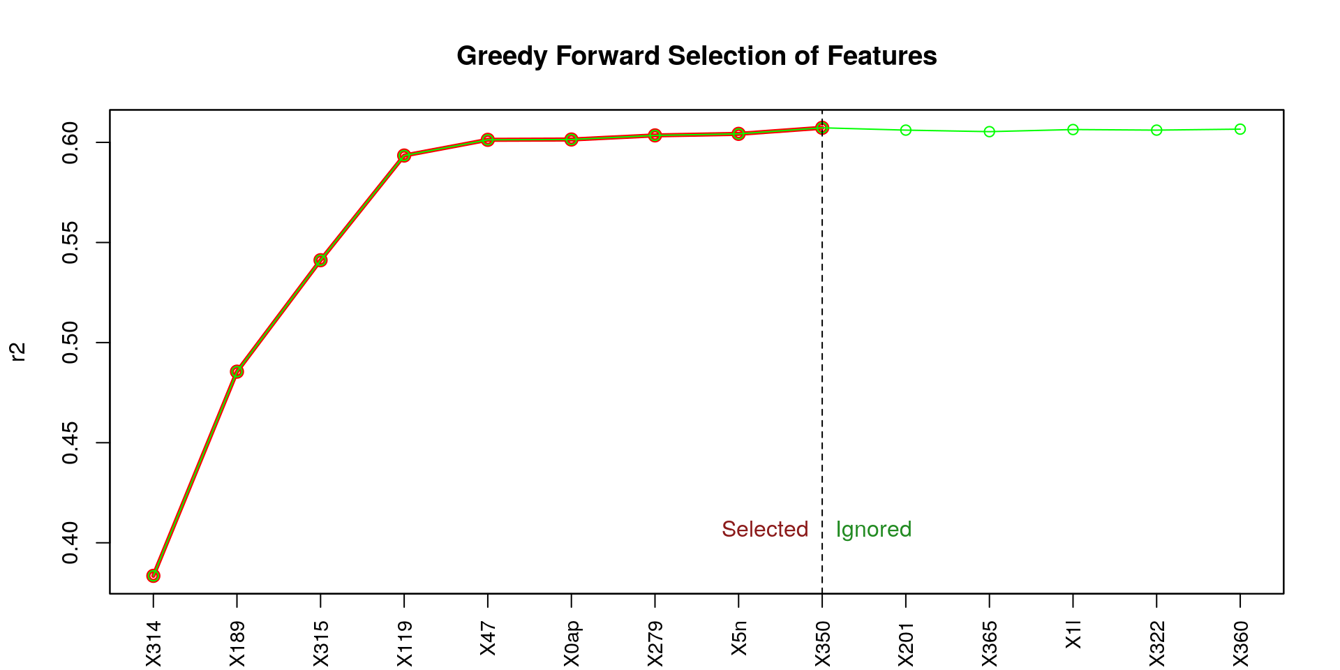
Here the set of selected features:
## [1] "X314" "X189" "X315" "X119" "X47" "X0ap" "X279" "X5n" "X350"
Selected Features & Gradient Boosting Machine
From the figure above (titled Greedy Forward Selection of Features), we can observe that the first four features (X314, X189, X315, X119) contribute the most to a high coefficient of determination (r2), and in a notable way. Let’s try to use those four feature only.
Note that we have also tried with:
- The first five features; although we got a better score on Kaggle’s LB than with only four features, the two scores remain somewhat comparable—0.55031 vs. 0.55123.
- The entire selected set of features (i.e., 9 features). We did not submit the results on the LB; however, the validation result suggests a comparable outcome with only four or five features.
Here we set the number of features we want to use.
numberOfFeatures <- 4 #5, length(selectedFeatures)
selectedFeatures <- selectedFeatures[1:numberOfFeatures]
Data sets preparation.
trainReduced <- convertInteger2Numeric(train[, c(selectedFeatures, "ID", response)])
validReduced <- convertInteger2Numeric(valid[, c(selectedFeatures, "ID", response)])
testReduced <- convertInteger2Numeric(test[, c(selectedFeatures, "ID", response)])
The three following vectors of indexes to ignore should be identical given that ID is consistently the first column and response the last one.
indexToIgnoreTrain <- c(grep(paste0("^", response, "$"), names(trainReduced)),
                        grep("^ID$", names(trainReduced)))

indexToIgnoreValid <- c(grep(paste0("^", response, "$"), names(validReduced)),
                        grep("^ID$", names(validReduced)))

indexToIgnoreTest <- c(grep(paste0("^", response, "$"), names(testReduced)),
                        grep("^ID$", names(testReduced)))
Models Selection (Grid Search) Using a Validation Set
hyperParams <- list ()

hyperParams$nround <- c(800)
hyperParams$eta <- c(0.01)
hyperParams$max_depth <- c(3, 4, 5)
hyperParams$gamma <- c(0)
hyperParams$colsample_bytree <- c(1) #c(0.75, 1)
hyperParams$min_child_weight <- c(1, 2, 3)
hyperParams$subsample <- c(0.7, 1)

gridSearchFsResult <- gridSearch (
  hyperParams = hyperParams,
  train = trainReduced, indexToIgnoreTrain = indexToIgnoreTrain,
  valid = validReduced, indexToIgnoreValid = indexToIgnoreValid,
  test = testReduced, indexToIgnoreTest = indexToIgnoreTest,
  response = response,
  verbose = TRUE)
Here is the head of the sorted grid result—decreasingly by validR2 (r2 achieved on the validation set); then, increasingly by trainR2 (r2 achieved on the training set). The column index is just a way for us to retrieve the prediction associated with the row.
> print(head(gridSearchFsResult$grid, 10), row.names = FALSE)
max_depth min_child_weight subsample validR2  trainR2 validMse trainMse index
    3                1       1.0 0.5952339 0.6057448 64.61462 58.67369    10
    3                3       0.7 0.5950666 0.6032525 64.64133 59.04460     7
    4                1       1.0 0.5950264 0.6059887 64.64773 58.63739    11
    5                1       1.0 0.5950264 0.6059887 64.64773 58.63739    12
    4                2       1.0 0.5950184 0.6052471 64.64902 58.74776    14
    5                2       1.0 0.5950184 0.6052471 64.64902 58.74776    15
    3                2       1.0 0.5949611 0.6052347 64.65816 58.74959    13
    4                3       0.7 0.5949598 0.6032832 64.65838 59.04003     8
    5                3       0.7 0.5949598 0.6032832 64.65838 59.04003     9
    4                3       1.0 0.5948493 0.6034408 64.67601 59.01657    17
A more extensive grid search could lead to improved performances, but we are quite limited in computational resources… It is worth noting that the small difference between the validation column (validR2) and the training column (trainR2) is rather a good sign (at least, it does not suggest a massive overfitting issue).
Retraining Best Models Using the Entire Training Set
We retrain the best model using the entire data set (i.e., rbind(train, valid)) and can submit the resulting predictions to Kaggle’s LB to see how well this model alone performs on the test set.
retrainModel <- function (xgb, train, valid, indexToIgnore, response, seed = 1) {
  set.seed(seed)
  xgbRetrained <- xgboost(
    data = data.matrix(
      rbind(train, valid)[, -indexToIgnore]),
    label = rbind(train, valid)[[response]],
    max.depth = xgb$params$max_depth,
    eta = xgb$params$eta,
    nround = xgb$niter,
    alpha = xgb$params$alpha,
    gamma = xgb$params$gamma,
    colsample_bytree = xgb$params$colsample_bytree,
    min_child_weight = xgb$params$min_child_weight,
    subsample = xgb$params$subsample,
    objective = xgb$params$objective,
    seed = seed,
    nthread = parallel:::detectCores(),
    verbose = TRUE,
    print_every_n = 200,
    save_period = NULL)
  return (xgbRetrained)
}
finalFsModel <- retrainModel(
  xgb = gridSearchFsResult$model,
  train = trainReduced,
  valid = validReduced,
  indexToIgnore = indexToIgnoreTrain,
  response = response,
  seed = gridSearchFsResult$model$params$seed)

resultRetrained <- predict(
  finalFsModel, data.matrix(testReduced[, -indexToIgnoreTest]))
saveResult(Xt$ID, result,
           paste0("result-fs-retrained_nfeatures-", numberOfFeatures, "_",
                  modelParam2String(gridSearchFsResult$model)))
Finally, we can average the first few top-ranked models’ predictions (we would expect a gain in performance).
numberOfModelsToAverage <- 6
averageAndSave <- function (ids, gridSearchResult, n, prefix, retrain = FALSE,
                            train = NULL, valid = NULL, test = NULL,
                            indexToIgnore = NULL, response = NULL) {
  grid <- gridSearchResult$grid
  nPred <- min(n, nrow(grid))
  predictions <- gridSearchResult$predictions
  models <- gridSearchResult$models
  for (i in 1:nPred) {
    if (!retrain) {
      preds <- predictions[[grid[i, ]$index]]
    } else {
      model <- models[[grid[i, ]$index]]
      retrainedModel <- retrainModel(
        xgb = model, train = train, valid = valid, indexToIgnore = indexToIgnore,
        response = response, seed = model$params$seed)

      preds <- predict(retrainedModel, data.matrix(test[, -indexToIgnore]))
    }
    if (i == 1) {
      aggregatedPredictions <- preds
    } else {
      aggregatedPredictions <- aggregatedPredictions + preds
    }
  }
  aggregatedPredictions <- aggregatedPredictions / nPred
  saveResult(ids, aggregatedPredictions, paste0(prefix, "n-", nPred))
  return (aggregatedPredictions)
}
Let’s also submit those predictions to Kaggle’s LB.
averageAndSave(
  Xt$ID, gridSearchFsResult, numberOfModelsToAverage,
  paste0("result-fs-agg_nfeatures-", numberOfFeatures, "_"),
  retrain = TRUE, valid = validReduced,
  train = trainReduced, test = testReduced,
  indexToIgnore = indexToIgnoreTrain, response = response)
License and Source Code
© 2017 Loic Merckel, Apache v2 licensed. The source code is available on both Kaggle and GitHub.
-
By basic features, we mean features that were there in the initial data set. ↩